CSC with a Spatial Mask
This example demonstrates the use of cbpdn.AddMaskSim for
convolutional sparse coding with a spatial mask
[50]. The example problem is inpainting of
randomly distributed corruption of a colour image
[51].
from __future__ import print_function
from builtins import input

import pyfftw   # See https://github.com/pyFFTW/pyFFTW/issues/40
import numpy as np

from sporco import util
from sporco import signal
from sporco import plot
plot.config_notebook_plotting()
from sporco.admm import tvl2
from sporco.admm import cbpdn
from sporco.metric import psnr
Load a reference image.
img = util.ExampleImages().image('monarch.png', zoom=0.5, scaled=True,
                                 idxexp=np.s_[:, 160:672])
Create random mask and apply to reference image to obtain test image.
(The call to numpy.random.seed ensures that the pseudo-random noise
is reproducible.)
np.random.seed(12345)
frc = 0.5
msk = signal.rndmask(img.shape, frc, dtype=np.float32)
imgw = msk * img
Define pad and crop functions.
pn = 8
spad = lambda x: np.pad(x, ((pn, pn), (pn, pn), (0, 0)), mode='symmetric')
zpad = lambda x: np.pad(x, ((pn, pn), (pn, pn), (0, 0)), mode='constant')
crop = lambda x: x[pn:-pn, pn:-pn]
Construct padded mask and test image.
mskp = zpad(msk)
imgwp = spad(imgw)
\(\ell_2\)-TV denoising with a spatial mask as a non-linear lowpass filter. The highpass component is the difference between the test image and the lowpass component, multiplied by the mask for faster convergence of the convolutional sparse coding (see [60]).
lmbda = 0.05
opt = tvl2.TVL2Denoise.Options({'Verbose': False, 'MaxMainIter': 200,
                    'DFidWeight': mskp, 'gEvalY': False,
                    'AutoRho': {'Enabled': True}})
b = tvl2.TVL2Denoise(imgwp, lmbda, opt, caxis=2)
sl = b.solve()
sh = mskp * (imgwp - sl)
Load dictionary.
D = util.convdicts()['RGB:8x8x3x64']
Set up admm.cbpdn.ConvBPDN options.
lmbda = 2e-2
opt = cbpdn.ConvBPDN.Options({'Verbose': True, 'MaxMainIter': 200,
                    'HighMemSolve': True, 'RelStopTol': 5e-3,
                    'AuxVarObj': False, 'RelaxParam': 1.8,
                    'rho': 5e1*lmbda + 1e-1, 'AutoRho': {'Enabled': False,
                    'StdResiduals': False}})
Construct admm.cbpdn.AddMaskSim wrapper for
admm.cbpdn.ConvBPDN and solve via wrapper. This example
could also have made use of admm.cbpdn.ConvBPDNMaskDcpl,
which has similar performance in this application, but
admm.cbpdn.AddMaskSim has the advantage of greater
flexibility in that the wrapper can be applied to a variety of CSC
solver objects.
ams = cbpdn.AddMaskSim(cbpdn.ConvBPDN, D, sh, mskp, lmbda, opt=opt)
X = ams.solve()
Itn   Fnc       DFid      Regℓ1     r         s
------------------------------------------------------
   0  3.61e+01  2.40e+00  1.69e+03  9.50e-01  6.10e-01
   1  3.42e+01  4.54e+00  1.48e+03  3.68e-01  5.88e-01
   2  2.96e+01  2.83e+00  1.34e+03  2.11e-01  2.91e-01
   3  2.73e+01  2.39e+00  1.24e+03  1.58e-01  1.98e-01
   4  2.61e+01  2.23e+00  1.19e+03  1.32e-01  1.50e-01
   5  2.53e+01  2.18e+00  1.16e+03  1.15e-01  1.21e-01
   6  2.43e+01  2.18e+00  1.11e+03  1.02e-01  1.04e-01
   7  2.35e+01  2.21e+00  1.06e+03  9.21e-02  9.08e-02
   8  2.27e+01  2.26e+00  1.02e+03  8.40e-02  8.07e-02
   9  2.22e+01  2.31e+00  9.93e+02  7.69e-02  7.22e-02
  10  2.17e+01  2.37e+00  9.67e+02  7.10e-02  6.53e-02
  11  2.13e+01  2.42e+00  9.42e+02  6.58e-02  5.96e-02
  12  2.08e+01  2.46e+00  9.15e+02  6.11e-02  5.48e-02
  13  2.02e+01  2.51e+00  8.87e+02  5.70e-02  5.06e-02
  14  1.97e+01  2.55e+00  8.59e+02  5.33e-02  4.68e-02
  15  1.92e+01  2.59e+00  8.32e+02  4.99e-02  4.37e-02
  16  1.88e+01  2.62e+00  8.07e+02  4.69e-02  4.10e-02
  17  1.83e+01  2.66e+00  7.84e+02  4.42e-02  3.84e-02
  18  1.80e+01  2.69e+00  7.64e+02  4.18e-02  3.59e-02
  19  1.76e+01  2.72e+00  7.45e+02  3.96e-02  3.38e-02
  20  1.73e+01  2.74e+00  7.27e+02  3.75e-02  3.18e-02
  21  1.70e+01  2.77e+00  7.11e+02  3.56e-02  2.99e-02
  22  1.67e+01  2.79e+00  6.96e+02  3.39e-02  2.82e-02
  23  1.65e+01  2.81e+00  6.83e+02  3.22e-02  2.66e-02
  24  1.62e+01  2.83e+00  6.70e+02  3.07e-02  2.52e-02
  25  1.60e+01  2.84e+00  6.58e+02  2.93e-02  2.38e-02
  26  1.58e+01  2.86e+00  6.47e+02  2.79e-02  2.27e-02
  27  1.56e+01  2.87e+00  6.36e+02  2.67e-02  2.16e-02
  28  1.54e+01  2.88e+00  6.25e+02  2.55e-02  2.06e-02
  29  1.52e+01  2.89e+00  6.16e+02  2.44e-02  1.97e-02
  30  1.50e+01  2.90e+00  6.06e+02  2.34e-02  1.89e-02
  31  1.49e+01  2.91e+00  5.98e+02  2.24e-02  1.81e-02
  32  1.47e+01  2.92e+00  5.91e+02  2.15e-02  1.73e-02
  33  1.46e+01  2.93e+00  5.84e+02  2.07e-02  1.65e-02
  34  1.45e+01  2.94e+00  5.78e+02  1.99e-02  1.57e-02
  35  1.44e+01  2.94e+00  5.72e+02  1.91e-02  1.51e-02
  36  1.42e+01  2.95e+00  5.65e+02  1.84e-02  1.45e-02
  37  1.41e+01  2.95e+00  5.59e+02  1.77e-02  1.39e-02
  38  1.40e+01  2.96e+00  5.52e+02  1.71e-02  1.34e-02
  39  1.39e+01  2.96e+00  5.47e+02  1.65e-02  1.29e-02
  40  1.38e+01  2.97e+00  5.41e+02  1.59e-02  1.25e-02
  41  1.37e+01  2.97e+00  5.36e+02  1.54e-02  1.20e-02
  42  1.36e+01  2.97e+00  5.32e+02  1.49e-02  1.16e-02
  43  1.35e+01  2.98e+00  5.27e+02  1.44e-02  1.12e-02
  44  1.34e+01  2.98e+00  5.23e+02  1.39e-02  1.09e-02
  45  1.34e+01  2.98e+00  5.19e+02  1.35e-02  1.05e-02
  46  1.33e+01  2.99e+00  5.15e+02  1.30e-02  1.02e-02
  47  1.32e+01  2.99e+00  5.11e+02  1.26e-02  9.88e-03
  48  1.31e+01  2.99e+00  5.07e+02  1.23e-02  9.56e-03
  49  1.31e+01  3.00e+00  5.04e+02  1.19e-02  9.23e-03
  50  1.30e+01  3.00e+00  5.01e+02  1.15e-02  8.93e-03
  51  1.30e+01  3.00e+00  4.98e+02  1.12e-02  8.65e-03
  52  1.29e+01  3.00e+00  4.95e+02  1.09e-02  8.37e-03
  53  1.28e+01  3.01e+00  4.92e+02  1.06e-02  8.12e-03
  54  1.28e+01  3.01e+00  4.89e+02  1.03e-02  7.86e-03
  55  1.27e+01  3.01e+00  4.86e+02  9.99e-03  7.61e-03
  56  1.27e+01  3.01e+00  4.83e+02  9.72e-03  7.37e-03
  57  1.26e+01  3.02e+00  4.81e+02  9.46e-03  7.15e-03
  58  1.26e+01  3.02e+00  4.79e+02  9.21e-03  6.94e-03
  59  1.25e+01  3.02e+00  4.76e+02  8.96e-03  6.74e-03
  60  1.25e+01  3.02e+00  4.74e+02  8.73e-03  6.56e-03
  61  1.25e+01  3.02e+00  4.72e+02  8.51e-03  6.38e-03
  62  1.24e+01  3.03e+00  4.70e+02  8.29e-03  6.22e-03
  63  1.24e+01  3.03e+00  4.68e+02  8.08e-03  6.05e-03
  64  1.23e+01  3.03e+00  4.66e+02  7.88e-03  5.89e-03
  65  1.23e+01  3.03e+00  4.64e+02  7.69e-03  5.75e-03
  66  1.23e+01  3.03e+00  4.62e+02  7.51e-03  5.62e-03
  67  1.22e+01  3.03e+00  4.60e+02  7.33e-03  5.49e-03
  68  1.22e+01  3.03e+00  4.58e+02  7.15e-03  5.37e-03
  69  1.21e+01  3.04e+00  4.56e+02  6.98e-03  5.25e-03
  70  1.21e+01  3.04e+00  4.54e+02  6.82e-03  5.13e-03
  71  1.21e+01  3.04e+00  4.52e+02  6.67e-03  5.01e-03
  72  1.21e+01  3.04e+00  4.51e+02  6.52e-03  4.90e-03
  73  1.20e+01  3.04e+00  4.49e+02  6.38e-03  4.79e-03
  74  1.20e+01  3.04e+00  4.48e+02  6.24e-03  4.69e-03
  75  1.20e+01  3.04e+00  4.46e+02  6.10e-03  4.60e-03
  76  1.19e+01  3.04e+00  4.45e+02  5.97e-03  4.50e-03
  77  1.19e+01  3.04e+00  4.44e+02  5.84e-03  4.42e-03
  78  1.19e+01  3.05e+00  4.42e+02  5.72e-03  4.33e-03
  79  1.19e+01  3.05e+00  4.41e+02  5.60e-03  4.25e-03
  80  1.18e+01  3.05e+00  4.40e+02  5.49e-03  4.17e-03
  81  1.18e+01  3.05e+00  4.38e+02  5.37e-03  4.10e-03
  82  1.18e+01  3.05e+00  4.37e+02  5.27e-03  4.02e-03
  83  1.18e+01  3.05e+00  4.36e+02  5.17e-03  3.94e-03
  84  1.18e+01  3.05e+00  4.35e+02  5.07e-03  3.86e-03
  85  1.17e+01  3.05e+00  4.34e+02  4.97e-03  3.78e-03
------------------------------------------------------
Reconstruct from representation.
imgr = crop(sl + ams.reconstruct().squeeze())
Display solve time and reconstruction performance.
print("AddMaskSim wrapped ConvBPDN solve time: %.2fs" %
      ams.timer.elapsed('solve'))
print("Corrupted image PSNR: %5.2f dB" % psnr(img, imgw))
print("Recovered image PSNR: %5.2f dB" % psnr(img, imgr))
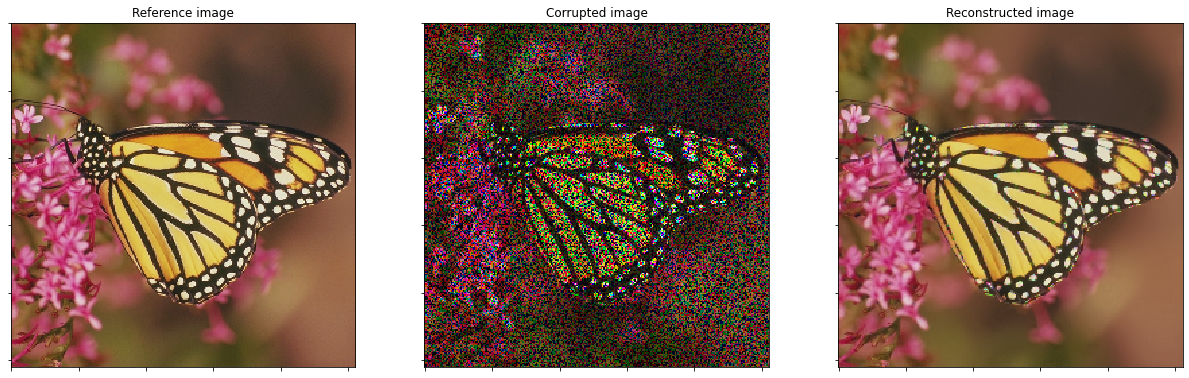
AddMaskSim wrapped ConvBPDN solve time: 42.42s
Corrupted image PSNR: 10.57 dB
Recovered image PSNR: 29.37 dB
Display reference, test, and reconstructed image
fig = plot.figure(figsize=(21, 7))
plot.subplot(1, 3, 1)
plot.imview(img, title='Reference image', fig=fig)
plot.subplot(1, 3, 2)
plot.imview(imgw, title='Corrupted image', fig=fig)
plot.subplot(1, 3, 3)
plot.imview(imgr, title='Reconstructed image', fig=fig)
fig.show()
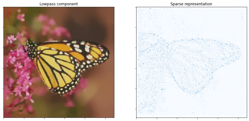
Display lowpass component and sparse representation
fig = plot.figure(figsize=(14, 7))
plot.subplot(1, 2, 1)
plot.imview(sl, cmap=plot.cm.Blues, title='Lowpass component', fig=fig)
plot.subplot(1, 2, 2)
plot.imview(np.squeeze(np.sum(abs(X), axis=ams.cri.axisM)),
            cmap=plot.cm.Blues, title='Sparse representation', fig=fig)
fig.show()
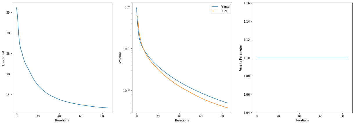
Plot functional value, residuals, and rho
its = ams.getitstat()
fig = plot.figure(figsize=(21, 7))
plot.subplot(1, 3, 1)
plot.plot(its.ObjFun, xlbl='Iterations', ylbl='Functional', fig=fig)
plot.subplot(1, 3, 2)
plot.plot(np.vstack((its.PrimalRsdl, its.DualRsdl)).T, ptyp='semilogy',
          xlbl='Iterations', ylbl='Residual', lgnd=['Primal', 'Dual'],
          fig=fig)
plot.subplot(1, 3, 3)
plot.plot(its.Rho, xlbl='Iterations', ylbl='Penalty Parameter', fig=fig)
fig.show()