Basis Pursuit DeNoising with Joint Sparsity
This example demonstrates the use of class bpdn.BPDNJoint to
solve the Basis Pursuit DeNoising (BPDN) problem with joint sparsity via
an \(ℓ_{2,1}\) norm term
where \(D\) is the dictionary, \(X\) is the sparse representation, and \(S\) is the signal to be represented. In this example the BPDN problem is used to estimate the reference sparse representation that generated a signal from a noisy version of the signal.
from __future__ import print_function
from builtins import input

import numpy as np

from sporco.admm import bpdn
from sporco import util
from sporco import plot
plot.config_notebook_plotting()
Configure problem size, sparsity, and noise level.
N = 32         # Signal size
M = 4*N        # Dictionary size
L = 12         # Number of non-zero coefficients in generator
K = 16         # Number of signals
sigma = 0.5    # Noise level
Construct random dictionary, reference random sparse representation, and test signal consisting of the synthesis of the reference sparse representation with additive Gaussian noise.
# Construct random dictionary and random sparse coefficients
np.random.seed(12345)
D = np.random.randn(N, M)
x0 = np.zeros((M, K))
si = np.random.permutation(list(range(0, M-1)))
x0[si[0:L],:] = np.random.randn(L, K)
# Construct reference and noisy signal
s0 = D.dot(x0)
s = s0 + sigma*np.random.randn(N,K)
Set BPDNJoint solver class options.
opt = bpdn.BPDNJoint.Options({'Verbose': False, 'MaxMainIter': 500,
                              'RelStopTol': 1e-3, 'rho': 10.0,
                              'AutoRho': {'RsdlTarget': 1.0}})
Select regularization parameters \(\lambda, \mu\) by evaluating the
error in recovering the sparse representation over a logarithmicaly
spaced grid. (The reference representation is assumed to be known, which
is not realistic in a real application.) A function is defined that
evalues the BPDN recovery error for a specified \(\lambda, \mu\),
and this function is evaluated in parallel by
sporco.util.grid_search.
# Function computing reconstruction error for (lmbda, mu) pair
def evalerr(prm):
    lmbda = prm[0]
    mu = prm[1]
    b = bpdn.BPDNJoint(D, s, lmbda, mu, opt)
    x = b.solve()
    return np.sum(np.abs(x-x0))


# Parallel evalution of error function on lmbda,mu grid
lrng = np.logspace(-4, 0.5, 10)
mrng = np.logspace(0.5, 1.6, 10)
sprm, sfvl, fvmx, sidx = util.grid_search(evalerr, (lrng, mrng))
lmbda = sprm[0]
mu = sprm[1]

print('Minimum ℓ1 error: %5.2f at (𝜆,μ) = (%.2e, %.2e)' % (sfvl, lmbda, mu))
Minimum ℓ1 error: 40.36 at (𝜆,μ) = (1.00e-04, 1.71e+01)
Once the best \(\lambda, \mu\) have been determined, run
bpdn.BPDNJoint.solve with verbose display of ADMM iteration
statistics.
# Initialise and run BPDNJoint object for best lmbda and mu
opt['Verbose'] = True
b = bpdn.BPDNJoint(D, s, lmbda, mu, opt)
x = b.solve()

print("BPDNJoint solve time: %.2fs" % b.timer.elapsed('solve'))
Itn   Fnc       DFid      Regℓ1     Regℓ2,1   r         s         ρ
--------------------------------------------------------------------------
   0  2.50e+03  2.44e+03  1.08e+01  3.18e+00  9.14e-01  1.43e-01  1.00e+01
   1  1.01e+03  5.79e+02  8.48e+01  2.55e+01  5.50e-01  3.77e-01  1.00e+01
   2  1.20e+03  4.44e+02  1.46e+02  4.39e+01  2.81e-01  3.51e-01  1.00e+01
   3  8.65e+02  1.72e+02  1.35e+02  4.05e+01  1.99e-01  2.26e-01  1.00e+01
   4  7.83e+02  1.76e+02  1.19e+02  3.55e+01  1.51e-01  1.96e-01  1.00e+01
   5  7.74e+02  2.04e+02  1.13e+02  3.33e+01  1.27e-01  1.00e-01  1.00e+01
   6  7.39e+02  1.54e+02  1.16e+02  3.42e+01  9.41e-02  7.47e-02  1.00e+01
   7  7.30e+02  1.08e+02  1.23e+02  3.63e+01  6.86e-02  7.00e-02  1.00e+01
   8  7.27e+02  9.87e+01  1.24e+02  3.67e+01  5.50e-02  4.15e-02  1.00e+01
   9  7.23e+02  1.12e+02  1.20e+02  3.57e+01  4.29e-02  3.56e-02  1.00e+01
  10  7.22e+02  1.21e+02  1.18e+02  3.51e+01  3.34e-02  2.73e-02  1.10e+01
  11  7.20e+02  1.09e+02  1.20e+02  3.57e+01  2.62e-02  2.32e-02  1.10e+01
  12  7.19e+02  9.89e+01  1.22e+02  3.63e+01  2.12e-02  1.72e-02  1.10e+01
  13  7.19e+02  1.01e+02  1.21e+02  3.61e+01  1.65e-02  1.05e-02  1.10e+01
  14  7.19e+02  1.05e+02  1.21e+02  3.59e+01  1.31e-02  9.99e-03  1.10e+01
  15  7.19e+02  1.05e+02  1.21e+02  3.59e+01  1.07e-02  7.80e-03  1.10e+01
  16  7.19e+02  1.01e+02  1.21e+02  3.61e+01  8.85e-03  5.53e-03  1.10e+01
  17  7.18e+02  1.01e+02  1.21e+02  3.61e+01  7.16e-03  3.25e-03  1.10e+01
  18  7.18e+02  1.02e+02  1.21e+02  3.60e+01  5.79e-03  3.35e-03  1.10e+01
  19  7.18e+02  1.02e+02  1.21e+02  3.60e+01  4.95e-03  2.53e-03  1.10e+01
  20  7.18e+02  1.01e+02  1.21e+02  3.61e+01  3.93e-03  1.73e-03  1.54e+01
  21  7.18e+02  1.01e+02  1.21e+02  3.61e+01  3.18e-03  1.78e-03  1.54e+01
  22  7.18e+02  1.01e+02  1.21e+02  3.61e+01  2.63e-03  1.60e-03  1.54e+01
  23  7.18e+02  1.01e+02  1.21e+02  3.61e+01  2.19e-03  1.07e-03  1.54e+01
  24  7.18e+02  1.01e+02  1.21e+02  3.61e+01  1.81e-03  8.09e-04  1.54e+01
  25  7.18e+02  1.01e+02  1.21e+02  3.61e+01  1.49e-03  7.34e-04  1.54e+01
  26  7.18e+02  1.01e+02  1.21e+02  3.61e+01  1.24e-03  5.96e-04  1.54e+01
  27  7.18e+02  1.01e+02  1.21e+02  3.61e+01  1.04e-03  4.27e-04  1.54e+01
  28  7.18e+02  1.01e+02  1.21e+02  3.61e+01  8.69e-04  3.11e-04  1.54e+01
--------------------------------------------------------------------------
BPDNJoint solve time: 0.01s
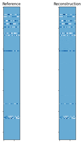
Plot comparison of reference and recovered representations.
fig = plot.figure(figsize=(6, 8))
plot.subplot(1, 2, 1)
plot.imview(x0, cmap=plot.cm.Blues, title='Reference', fig=fig)
plot.subplot(1, 2, 2)
plot.imview(x, cmap=plot.cm.Blues, title='Reconstruction', fig=fig)
fig.show()
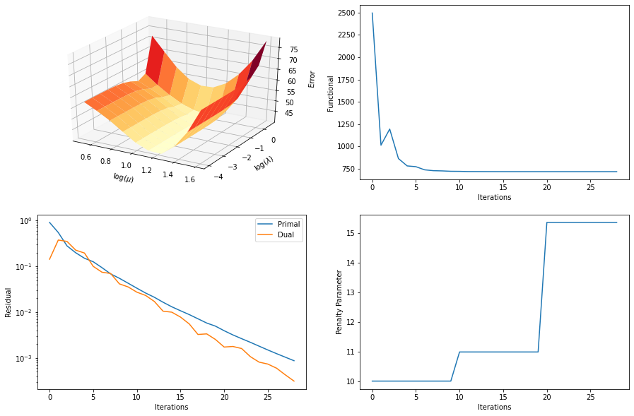
Plot lmbda, mu error surface, functional value, residuals, and rho
its = b.getitstat()
fig = plot.figure(figsize=(15, 10))
ax = fig.add_subplot(2, 2, 1, projection='3d')
ax.locator_params(nbins=5, axis='y')
plot.surf(fvmx, x=np.log10(mrng), y=np.log10(lrng), xlbl=r'log($\mu$)',
          ylbl=r'log($\lambda$)', zlbl='Error', fig=fig, ax=ax)
plot.subplot(2, 2, 2)
plot.plot(its.ObjFun, xlbl='Iterations', ylbl='Functional', fig=fig)
plot.subplot(2, 2, 3)
plot.plot(np.vstack((its.PrimalRsdl, its.DualRsdl)).T,
          ptyp='semilogy', xlbl='Iterations', ylbl='Residual',
          lgnd=['Primal', 'Dual'], fig=fig)
plot.subplot(2, 2, 4)
plot.plot(its.Rho, xlbl='Iterations', ylbl='Penalty Parameter', fig=fig)
fig.show()